9.12. Case Study HTML GDP

• https://pl.wikipedia.org/wiki/Lista_pa%C5%84stw_%C5%9Bwiata_wed%C5%82ug_PKB_nominalnego

• https://pl.wikipedia.org/wiki/Lista_pa%C5%84stw_%C5%9Bwiata_wed%C5%82ug_liczby_ludno%C5%9Bci

9.12.1. Case Study - 1

"""
>>> result.loc['Polska']
PKB          6.741270e+11
Ludność      3.842069e+07
PerCapita    1.754594e+04
Name: Polska, dtype: float64
"""

# %% Run
# - PyCharm: right-click in the editor and `Run Doctest in ...`
# - PyCharm: keyboard shortcut `Control + Shift + F10`
# - Terminal: `python -m doctest -f -v myfile.py`

# %% Imports
import pandas as pd
import matplotlib.pyplot as plt

# %% Types

# %% Data


pd.set_option('display.width', 200)
pd.set_option('display.max_columns', 15)
pd.set_option('display.max_rows', 100)
pd.set_option('display.min_rows', 100)
pd.set_option('display.max_seq_items', 100)


USD = 1

# PKB = 'https://pl.wikipedia.org/wiki/Lista_pa%C5%84stw_%C5%9Bwiata_wed%C5%82ug_PKB_nominalnego'
PKB = 'https://python3.info/_static/percapita-pkb.html'

# LUDNOSC = 'https://pl.wikipedia.org/wiki/Lista_pa%C5%84stw_%C5%9Bwiata_wed%C5%82ug_liczby_ludno%C5%9Bci'
LUDNOSC = 'https://python3.info/_static/percapita-ludnosc.html'

LUDNOSC_PANSTWA = {
    'Chińska Republika Ludowa': 'Chiny',
    'Korea Północna': pd.NA,
    'Republika Chińska': 'Tajwan',
    'Kuba': pd.NA,
    'Zachodni Brzeg': pd.NA,
    'Strefa Gazy': pd.NA}

LUDNOSC_COLUMNS = {
    'Państwo, obszar lub terytorium zależne': 'Państwo',
    '2018': 'Ludność'}


def clean(column):
    return (column
        .str.replace('\xa0', '')
        .str.replace(' ', ''))

pkb = (pd
    .read_html(PKB)[1]
    .rename(columns={'2021 r.': 'PKB'})
    .loc[:, ['Państwo', 'PKB']]
    .replace('b.d.', pd.NA)
    .dropna(how='any', axis='rows')
    .apply(clean)
    .astype({'PKB': 'int64'})
    .set_index('Państwo')
    .mul(1_000_000*USD))

ludnosc = (pd
    .read_html(LUDNOSC)[0]
    .droplevel(level=0, axis='columns')
    .rename(columns=LUDNOSC_COLUMNS)
    .loc[:, ['Państwo', 'Ludność']]
    .replace(LUDNOSC_PANSTWA)
    .set_index('Państwo')
    .query('index in @pkb.index')
    .apply(clean)
    .astype({'Ludność': 'int64'}))

result = (pkb
    .merge(ludnosc, left_index=True, right_index=True)
    .sort_index(ascending=True)
    .eval('PerCapita = PKB / Ludność'))

plot = (result
    .loc[:, ['PerCapita']]
    .round({'PerCapita': 1})
    .sort_values('PerCapita', ascending=False)
    .head(n=30)
    .plot(kind='bar', legend=True, grid=True, figsize=(16,10)))

# plt.show()

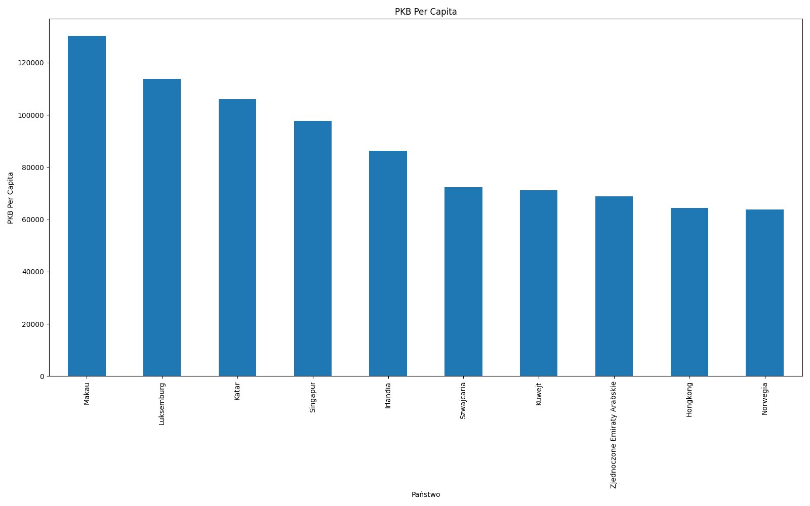
Figure 9.11. Top 10 countries with highest Global Domestic Product Per Capita

9.12.2. Case Study - 2

import pandas as pd
import matplotlib.pyplot as plt


pd.set_option('display.width', 80)
pd.set_option('display.max_rows', 200)
pd.set_option('display.max_columns', 10)
pd.set_option('display.max_colwidth', 100)

USD = 1

# PKB = 'https://pl.wikipedia.org/wiki/Lista_pa%C5%84stw_%C5%9Bwiata_wed%C5%82ug_PKB_nominalnego'
# LUDNOSC = 'https://pl.wikipedia.org/wiki/Lista_pa%C5%84stw_%C5%9Bwiata_wed%C5%82ug_liczby_ludno%C5%9Bci'
PKB = 'https://python3.info/_static/html-gdp-pkb.html'
LUDNOSC = 'https://python3.info/_static/html-gdp-ludnosc.html'

pkb = (
    pd
    .read_html(PKB)[2]
    .rename(columns={'Państwo':'kraj', '2022 r.':'pkb'})
    .loc[:, ['kraj', 'pkb']]
    .replace({'pkb': {'b.d.':pd.NA, ' ':''}}, regex=True)
    .astype({'kraj': 'string', 'pkb': 'Int64'})
    .convert_dtypes()
    .dropna()
    .set_index('kraj', drop=True)
    .mul(1_000_000*USD))

ludnosc = (
    pd
    .read_html(LUDNOSC)[0]
    .droplevel(0, axis='columns')
    .rename(columns={'Państwo, obszar lub terytorium zależne': 'kraj', '2022': 'ludnosc'})
    .loc[:, ['kraj', 'ludnosc']]
    .replace({'ludnosc': {'\xa0':'', r'\[3\]':'', ' ':'', '–':pd.NA}}, regex=True)
    .replace({'kraj': {'Chińska Republika Ludowa': 'Chiny'}})
    .dropna()
    .astype({'kraj': 'string', 'ludnosc': 'Int64'})
    .convert_dtypes()
    .set_index('kraj', drop=True)
    .query('index in @pkb.index'))

data = (
    pkb
    .join(ludnosc)
    .assign(per_capita=lambda df: df.pkb/df.ludnosc)
    .round({'per_capita': 2})
    .astype({'pkb': 'Int64', 'ludnosc': 'Int64', 'per_capita': 'Float64'})
    .convert_dtypes()
    .dropna()
    .sort_values('per_capita', ascending=False))

top_10_percapita = (
    data
    .head(10)
    .loc[:, ['per_capita']]
    .sort_values('per_capita')
).plot(
    title='Top 10 krajów wg PKB na mieszkańca',
    xlabel='Country',
    ylabel='USD Per Capita',
    kind='bar',
    legend=False,
    figsize=(20, 10),
)

plt.tight_layout()
plt.show()

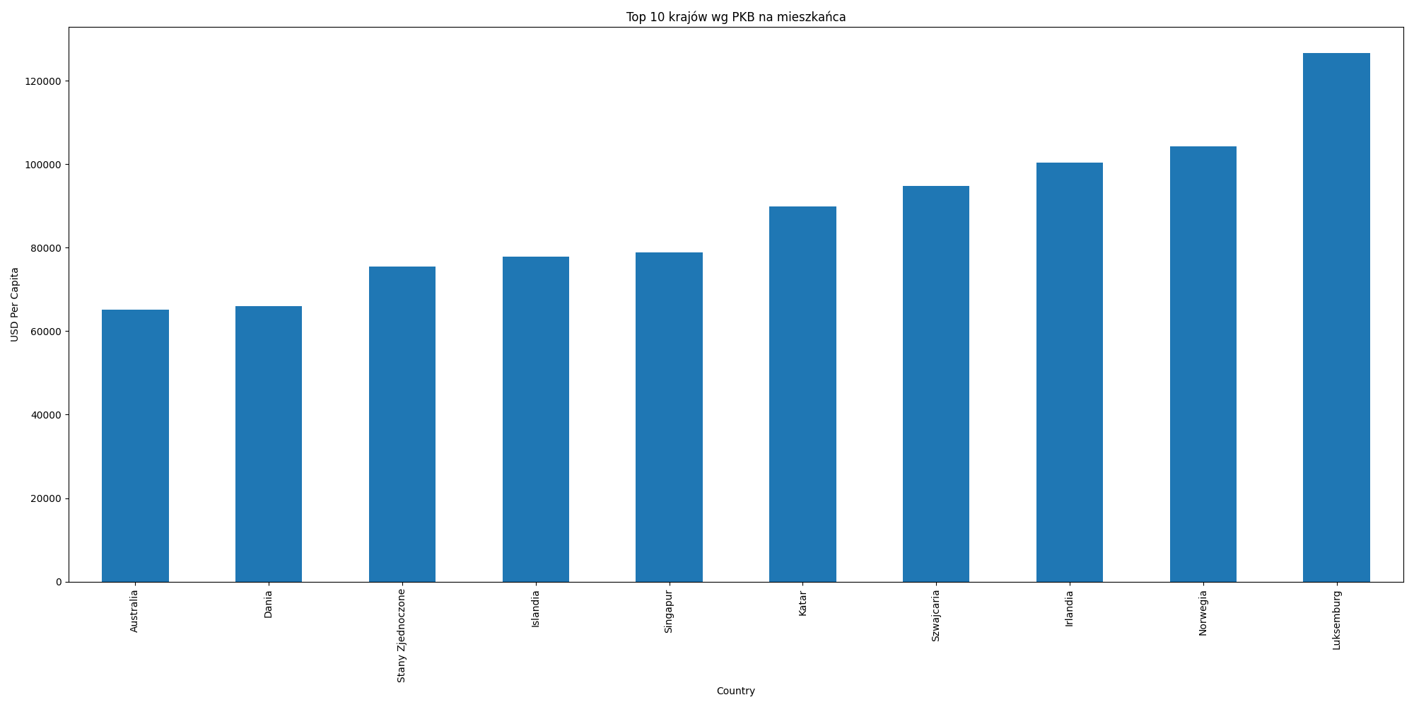
Figure 9.12. Top 10 countries with highest Global Domestic Product Per Capita

9.12.3. Case Study - 3

# %%

import pandas as pd
from matplotlib import pyplot as plt

pd.set_option('display.width', 500)
pd.set_option('display.max_columns', 10)
pd.set_option('display.max_rows', 500)

# %%

PKB = 'https://pl.wikipedia.org/wiki/Lista_pa%C5%84stw_%C5%9Bwiata_wed%C5%82ug_PKB_nominalnego'
LUDNOSC = 'https://pl.wikipedia.org/wiki/Lista_pa%C5%84stw_%C5%9Bwiata_wed%C5%82ug_liczby_ludno%C5%9Bci'

USD = 1

# %%

pkb = (
    pd
    .read_html(PKB)[3]
    .rename(columns={'Państwo':'kraj', '2021 r.':'pkb'})
    .loc[:, ['kraj', 'pkb']]
    .replace({'pkb': {'\xa0': '', 'b.d.': pd.NA}}, regex=True)
    .dropna(how='any', axis='rows')
    .astype({'kraj': 'str', 'pkb': 'int64'})
    .convert_dtypes()
    .set_index('kraj', drop=True)
    .drop(['Strefa euro', 'Wyspy Kokosowe', 'Palestyna'], axis='rows')
    .mul(1_000_000*USD)
)

# %%

ludnosc = (
    pd
    .read_html(LUDNOSC)[0]
    .droplevel(0, axis='columns')
    .rename(columns={'Państwo, obszar lub terytorium zależne':'kraj', '2022':'ludnosc'})
    .loc[:, ['kraj', 'ludnosc']]
    .replace({'ludnosc': {'\xa0': '', ' ': '', '–': pd.NA, r'\[3\]': ''}}, regex=True)
    .replace({'Chińska Republika Ludowa':'Chiny'})
    .dropna(how='any', axis='rows')
    .astype({'kraj': 'str', 'ludnosc': 'int64'})
    .convert_dtypes()
    .set_index('kraj', drop=True)
)

# %%

pkb.query('index not in @ludnosc.index')

# %%

result = (
    pd
    .concat([pkb, ludnosc], axis='columns', join='inner')
    .assign(per_capita=lambda df: df['pkb'] / df['ludnosc'])
    .round({'per_capita': 2})
    .convert_dtypes()
    .sort_values(by='per_capita', ascending=False)
)

# %%

plot_top10 = (
    result
    .head(10)
    .loc[:, ['per_capita']]
    .plot(
        kind='bar',
        title='Top 10 countries by GDP per capita',
        xlabel='Country',
        ylabel='GDP per capita [USD]',
        grid=False,
        figsize=(15,10),
        color='green')
)

plt.tight_layout()
plt.show()

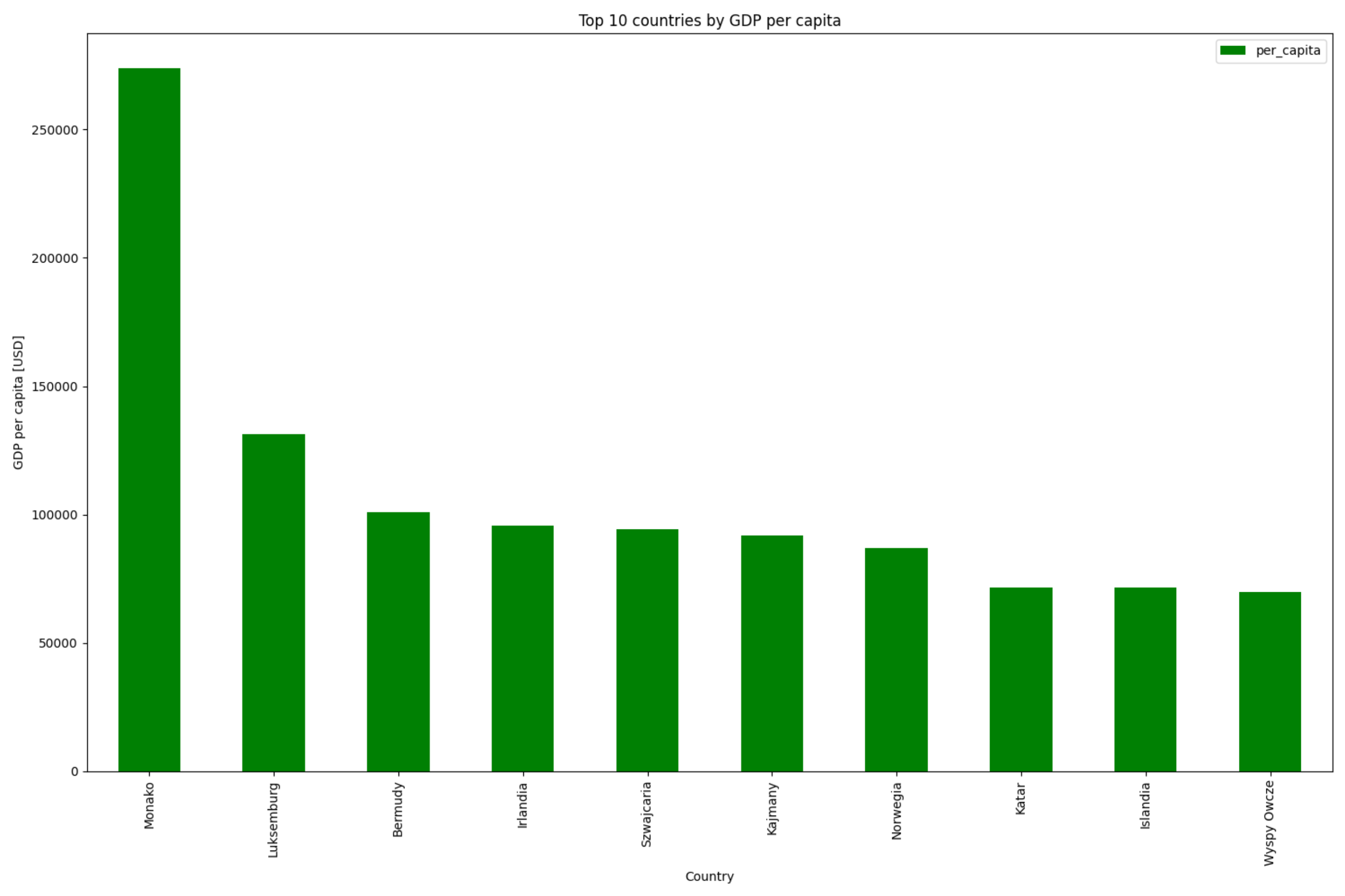
Figure 9.13. Top 10 countries with highest Global Domestic Product Per Capita

9.12.4. Case Study - 4

import pandas as pd
import matplotlib.pyplot as plt
from matplotlib.ticker import FuncFormatter

pd.set_option('display.max_columns', 50)
pd.set_option('display.max_rows', 300)
pd.set_option('display.width', 500)
pd.set_option('display.memory_usage', 'deep')
pd.set_option('display.precision', 4)

GDP = 'https://en.wikipedia.org/wiki/List_of_countries_by_GDP_(nominal)'
POPULATION = 'https://en.wikipedia.org/wiki/List_of_countries_and_dependencies_by_population'

# GDP = '/Users/matt/Developer/2025-11-pythonana-sages/_Trener/51-casestudies/03-gdp/data/gdp.html'
# POPULATION = '/Users/matt/Developer/2025-11-pythonana-sages/_Trener/51-casestudies/03-gdp/data/population.html'

USD = 1

COUNTRY = {
    'Hong Kong (China)': 'Hong Kong',
    'Puerto Rico (US)': 'Puerto Rico',
    'Macau (China)': 'Macau',
    'Aruba (Netherlands)': 'Aruba',
    'Democratic Republic of the Congo': 'DR Congo',
    'Republic of the Congo': 'Congo',
    'Curaçao (Netherlands)': 'Curaçao',
    'Guam (US)': 'Guam',
    'Jersey (UK)': 'Jersey',
    'U.S. Virgin Islands (US)': 'U.S. Virgin Islands',
    'Cayman Islands (UK)': 'Cayman Islands',
    'Isle of Man (UK)': 'Isle of Man',
    'Guernsey (UK)': 'Guernsey',
    'Bermuda (UK)': 'Bermuda',
    'Greenland (Denmark)': 'Greenland',
    'Faroe Islands (Denmark)': 'Faroe Islands',
    'Turks and Caicos Islands (UK)': 'Turks and Caicos Islands',
    'American Samoa (US)': 'American Samoa',
    'Northern Mariana Islands (US)': 'Northern Mariana Islands',
    'Sint Maarten (Netherlands)': 'Sint Maarten',
    'British Virgin Islands (UK)': 'British Virgin Islands',
    'Gibraltar (UK)': 'Gibraltar',
    'Saint Martin (France)': 'Saint Martin',
    'Anguilla (UK)': 'Anguilla',
    'Cook Islands (New Zealand)': 'Cook Islands',
    'Wallis and Futuna (France)': 'Wallis and Futuna',
    'Saint Barthélemy (France)': 'Saint Barthélemy',
    'Saint Pierre and Miquelon (France)': 'Saint Pierre and Miquelon',
    'Saint Helena, Ascension and Tristan da Cunha (UK)': 'Saint Helena',
    'Montserrat (UK)': 'Montserrat',
    'Falkland Islands (UK)': 'Falkland Islands',
    'Tokelau (New Zealand)': 'Tokelau',
    'Norfolk Island (Australia)': 'Norfolk Island',
    'Christmas Island (Australia)': 'Christmas Island',
    'Niue (New Zealand)': 'Niue',
    'Cocos (Keeling) Islands (Australia)': 'Cocos Islands',
    'Pitcairn Islands (UK)': 'Pitcairn Islands',
    'French Polynesia (France)': 'French Polynesia',
    'New Caledonia (France)': 'New Caledonia',
    'Western Sahara (disputed)': 'Western Sahara',
}

REMOVE = [
    'Yemen',
    'North Korea',
    'Syria',
    'Cuba',
    'Eritrea',
    'Western Sahara',
    'Northern Cyprus',
    'Transnistria',
    'French Polynesia',
    'New Caledonia',
    'Abkhazia',
    'Curaçao',
    'Guam',
    'Jersey',
    'U.S. Virgin Islands',
    'Cayman Islands',
    'Isle of Man',
    'Guernsey',
    'Bermuda',
    'Greenland',
    'South Ossetia',
    'Faroe Islands',
    'Turks and Caicos Islands',
    'American Samoa',
    'Northern Mariana Islands',
    'Sint Maarten',
    'British Virgin Islands',
    'Monaco',
    'Gibraltar',
    'Saint Martin',
    'Anguilla',
    'Cook Islands',
    'Wallis and Futuna',
    'Saint Barthélemy',
    'Saint Pierre and Miquelon',
    'Saint Helena',
    'Montserrat',
    'Falkland Islands',
    'Tokelau',
    'Norfolk Island',
    'Christmas Island',
    'Niue',
    'Vatican City',
    'Cocos Islands',
    'Pitcairn Islands',
]

# %% Load GDP data

gdp = (
    pd
    .read_html(GDP, storage_options={'User-Agent': 'My Browser'})[2]
    .rename(columns={'Country/Territory': 'country', 'IMF (2025)[6]': 'gdp'})
    .loc[:, ['country', 'gdp']]
    .replace({'country': {r'\[.+?\]':''}, 'gdp': {'—N/a': pd.NA, r',':'', r'\(\d{4}\)': ''}}, regex=True)
    .astype({'country': 'string', 'gdp': 'Int64'})
    .convert_dtypes(dtype_backend='pyarrow')
    .dropna(subset=['gdp'])
    .replace({'country': COUNTRY})
    .set_index('country', drop=True)
    .multiply(1_000_000*USD)
)

# %% Load Population data

population = (
    pd
    .read_html(POPULATION, storage_options={'User-Agent': 'My Browser'})[0]
    .rename(columns={'Location': 'country', 'Population': 'population'})
    .loc[:, ['country', 'population']]
    .convert_dtypes(dtype_backend='pyarrow')
    .replace({'country': COUNTRY})
    .set_index('country', drop=True)
    .drop(index=REMOVE)
)

# %% Merge

df = (
    pd
    .concat([gdp, population], axis='columns', join='inner')
    .assign(percapita=lambda df: df['gdp'] / df['population'])
    .convert_dtypes(dtype_backend='pyarrow')
    .sort_values(by='percapita', ascending=False)
    .round({'percapita': 2})
)

# %% Visualize

data = (
    df
    .head(10)
    .sort_values(by='percapita', ascending=True)
    .loc[:, ['percapita']]
)

ax = data.plot(
    kind='barh',
    title='Top 10 Countries by GDP per Capita (2025)',
    xlabel='GDP per Capita (USD)',
    ylabel='Country',
    color='blue',
    figsize=(10, 6),
    legend=False,
)

def format_thousands(x, pos=None):
    """Format numbers with 'k' for thousands"""
    if x >= 1000:
        return f'${x/1000:.0f}k'
    return f'${x:.0f}'

ax.xaxis.set_major_formatter(FuncFormatter(format_thousands))

for i, (country, value) in enumerate(data['percapita'].items()):
    ax.text(value, i, f' {format_thousands(value)}', va='center', fontsize=9)

globalmean = df['percapita'].mean()
top10mean = data['percapita'].mean()
ax.axvline(globalmean, color='red', linestyle='--', label=f'Global Mean: ${globalmean:,.2f}')
ax.axvline(top10mean, color='green', linestyle='--', label=f'Top 10 Mean: ${top10mean:,.2f}')
ax.legend()

plt.tight_layout()
plt.show()

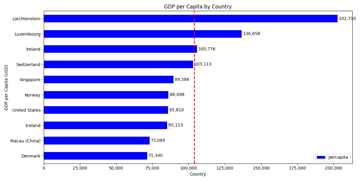
Figure 9.14. Top 10 countries with highest Global Domestic Product Per Capita